One question that every medical device manufacturer and health tech company building a medical AI solution asks is: how much data do I need to train my model?
The question sounds simple, but it is not. Four different questions are usually hiding inside it, and they have different answers:
- How much do I have to spend to achieve my objective? The objective is almost always the same shape: a model performant enough to support the claim the business wants to make, built without spending more than the product is worth.
- How do I get more data if I do not have enough? Sourcing, partnerships, licensing, and augmentation are a separate problem. They are out of scope here and will be treated in a future article.
- I know I need a lot of data, but do I need to have all of it at once? No. Treating the requirement as one purchase, made once, is the most expensive version of this mistake.
- How many samples do I need exactly? A number does exist. It becomes computable only after an intended-use claim, a primary endpoint, and a tolerated statistical uncertainty exist.
This article answers all four, within the scope below.
Scope of this article
- The subject is AI Software as a Medical Device (SaMD), software whose output is intended to inform or drive a clinical decision.
- It also covers clinical-workflow software that is not itself designated a medical device: research tools, data-analysis systems, and laboratory or operational analytics used inside the clinical process. The regulatory obligations differ, but the data-planning logic is the same, and these systems are frequently the on-ramp to a later regulated product.
- The focus is predictive analytic models: classification, detection, segmentation, measurement, and risk scoring.
- Generative models are out of scope and will be treated separately. Open-ended output, the absence of a single fixed reference standard, and the absence of one operating point break most of the sizing methods used below.
One counting rule applies throughout. Every number here refers to the independent unit defined by the intended use, usually the patient or the clinical case, not the number of images, patches, slices, frames, notes, or augmented copies. Repeated observations from the same patient add information, but they do not add independent clinical sample size one-for-one, and treating them as if they do is a common source of both overestimated datasets and inflated performance.
The simple answer: "as much as possible"
This is technically defensible and practically useless. It fails for six reasons.
It answers none of the four questions above. A team that asks for a budget, a timeline, and a sample count is told to maximise an unbounded quantity. Nothing in that reply can be planned against.
Data is scarce, and the scarcity is structural rather than incidental. A JAMA analysis of US cohorts used to train diagnostic deep-learning algorithms found that 40 of 56 studies with geographically identifiable cohorts, 71%, relied on patient data from California, Massachusetts, or New York, while 34 states contributed no cohorts at all. The world's supply of medical training data is not evenly distributed, and the parts of it that match a given intended-use population may barely exist.
Available data is messy. Willemink and colleagues, writing in Radiology, estimate that preprocessing and organising data for ingestion accounts for 80% or more of the effort in a medical imaging machine learning project. Raw volume in a PACS, an LIS, or an EHR is not the same as usable, labelled, legally cleared, leakage-free training data.
Good data is expensive. The same paper describes expert manual labelling of large populations as extremely time-consuming and costly, particularly for CT, PET, and MRI. Reference standards that require biopsy, adjudication, or outcome follow-up are more expensive still, and they are exactly the reference standards a claim usually needs.
Companies must plan and budget ahead. "As much as possible" cannot be entered on a budget line, placed on a Gantt chart, defended to a board, or written into a data-sharing agreement. It also cannot be used to decide whether the project should start at all.
It is not an engineering answer. It gives no stopping rule, no gate, and no way to know whether the next 5,000 cases will change anything.
So how much do we need really? It depends
Two facts settle a lot of arguments before they start.
No regulator prescribes a training-set size. IMDRF N41, the final IMDRF N88 good machine learning practice principles, MDCG 2020-1, MDCG 2025-6 / AIB 2025-1, and FDA's AI-enabled device lifecycle draft guidance all require training, validation, and test data that are representative, adequately sized, and justified. None of them names an N. The obligation is to defend the size you chose, not to hit a published threshold.
There is no single accepted standard either. Professional bodies publish heuristics. An IFCC working group cites roughly 1,000 to 5,000 examples per class as a rough rule for complex computer-vision and deep-learning tasks, but the same recommendation tells teams to measure learning curves rather than trust the range.
One qualification matters, because "no regulator requires a number" is often overstated. Evidence-type-specific guidance can still recommend counts. FDA's human factors and usability guidance generally recommends at least 15 representative participants per distinct user population for validation testing. The absence of a training-set minimum is not the absence of all numbers.
What the requirement actually depends on falls into four groups.
Objective
The data requirement is set by what the model has to be, not by what is available. The model should be stable, so performance does not swing with a different seed, fold, or resampling. It should be generalizable, which is bought with diversity rather than repetition. It has to cover the variation inside its own intended use: every scanner, protocol, preparation method, demographic group, and disease subtype named in the claim is a coverage obligation. It has to generate evidence, because a claim requires a study and a study requires enough target events. And it has to meet target metrics: a device that must reach 95% sensitivity needs more, and more carefully chosen, data than one that must reach 80%.
Stage of project
Training from scratch or building on a pretrained model changes the requirement by an order of magnitude. High-capacity models trained from random initialisation on imaging, signal, or language data usually need far more development data than a transfer-learned or conventional model on the same task.
Licence and permission determine how much of the data you can actually use. Consent basis, secondary-use rights, commercial-use rights, cross-border transfer, and the right to retain data for future retraining are all capable of removing a dataset from the plan after it has been counted.
System in place at the company
In-house development means the acquisition, annotation, and versioning burden sits with the team, so the requirement is bounded by what that team can process rather than by what exists. Outsourced development shifts execution but not accountability: the manufacturer still has to demonstrate provenance, label quality, and independence of the test data.
Data lifecycle management know-how is the quiet determinant. Teams that cannot version a dataset, trace a label back to its annotator, or prove that a test case never touched training will need more data than teams that can, because they lose cohorts to leakage, redo annotation rounds, and cannot reuse earlier evidence.
Task
Classification is generally the cheapest per case: one label per unit, and sizing follows binomial precision on the target class. Localization and measurement, meaning detection and segmentation, cost more, because annotation is spatial rather than categorical and because multiple correlated lesions within one patient complicate both labelling and analysis. Explanation and free-text output is a generative use case and is out of scope here.
What is needed instead of a number
Four artefacts replace the single figure. They are ordered deliberately: the method comes before the schedule, because the schedule is nothing more than the method applied stage by stage.
- A data budget, not a number. The matrix of what has to be collected and why.
- Evidence targets per stage. The metric, the sizing method that matches the question, and the tolerated statistical uncertainty, which together make a count computable.
- A timeline. Those targets placed against decision gates, so each count comes due when it is needed and not before.
- Diversity, label quality, and risk over volume. The corrections that no count can supply.
Artefact 01. A data budget, not a number
A data budget is a matrix, not a scalar. It maps every intended-use boundary and every risk control to a source, a case count, a target-event count, a label method, and a planned analysis. It also separates five buckets that regulators evaluate separately and that teams routinely blend into one.
| Bucket | What it is for |
|---|---|
| Development and training data | Fit model parameters or rules. |
| Tuning and internal validation | Select architecture, thresholds, features, and preprocessing. The moment data influence a choice, they become development data. |
| Locked analytical test data | Estimate standalone technical performance, independent at the patient, acquisition, and site levels the claim requires. |
| Clinical performance and human factors | Test the finished device in the intended population, workflow, and human-AI team. A prospective study, reader study, outcome study, or usability validation may be required, and no algorithm test set substitutes for it. |
| Post-market and change validation | Monitor real-world performance and support controlled modification. New versions need fresh or demonstrably sequestered test evidence. |
A budget expressed this way survives contact with a data-sharing negotiation. A single number does not.
Artefact 02. Evidence targets per stage: metrics and statistical uncertainty
This is where the requested number finally appears, and it appears for the validation study rather than the training set.
First identify the denominator for each metric. Sensitivity is true positives / all reference-standard-positive cases, so its precision is driven by the number of people who actually have the target condition. Specificity is true negatives / all reference-standard-negative cases, so its precision is driven by the number who do not. A study with 1,000 participants can still be far too small for a sensitivity claim if only a handful of them have the condition. FDA's diagnostic-test statistical guidance defines these denominators and recommends reporting the underlying fractions, percentages, and two-sided 95% confidence intervals.
Then pick the method that matches the question the study has to answer. There is no single sample-size formula for medical AI, and choosing one before deciding what the study must demonstrate is the most common way to arrive at a defensible-looking number that answers nothing.
Related work
Precision-based estimation. Buderer (1996) remains the reference point. Its contribution was to fold prevalence into the sizing of a diagnostic accuracy study, so that a required count of target-positive cases converts into a number of patients to recruit rather than staying an abstract event count. Its limitations are all consequences of its simplicity: it uses the Wald normal approximation, which is least trustworthy at the high expected performance and modest event counts typical of medical AI; it sizes a symmetric confidence-interval width rather than a decision; it sizes sensitivity and specificity as though they were separate studies; and it assumes prevalence is known rather than estimated.
Whittle et al. (2025) generalise that closed form to the full set of metrics a thresholded classifier reports, including accuracy, sensitivity, specificity, and positive and negative predictive value, together with an iterative procedure for the F1 score, implemented in the pmvalsampsize package. The novelty is coverage: one framework sizes every metric a submission is likely to quote. The limitation is that it remains an estimation-precision framing, and the authors are explicit that for sensitivity alone it reduces to the same binomial calculation as Buderer. It is an extension, not a replacement.
Monti, Ambrogi and Sardanelli (2024) provide the most useful single entry point, covering reliability sizing (Cohen's kappa, the intraclass correlation coefficient, Bland-Altman limits of agreement) alongside diagnostic performance, area under the ROC curve, and paired versus unpaired comparisons, each with worked examples. Its value is breadth rather than new methodology; it consolidates existing closed forms and does not address clustering, adaptive designs, or model-based validation.
Testing against a performance goal. Stark and Zapf (2020) address the question a confirmatory study actually asks, which is not how wide the interval will be but whether the device clears a prespecified minimum. Two features make it more applicable to a regulated submission than any precision calculation. Sensitivity and specificity are treated as genuine co-primary endpoints, so the study is powered for both passing rather than for each passing separately. And because the required sample depends heavily on an assumed prevalence, the authors add a one-time blinded re-estimation of prevalence during the study, which prevents a wrong initial assumption from producing a study that is overpowered in one subpopulation and underpowered in the other. The limitations are scope: it addresses the single-arm confirmatory setting with a fixed reference standard, and the interim re-estimation has to be prespecified rather than added later.
Validating a probability-output model. Riley et al. (2021) shift the target from accuracy to the properties that decide whether a risk model is usable: calibration-in-the-large, calibration slope, discrimination, and net benefit, with the required sample being the largest across the prespecified metrics. This matters because a model can discriminate well and still be miscalibrated badly enough to be unsafe at its operating threshold, a failure a sensitivity calculation cannot see. The practical limitation is that the closed forms need an assumed distribution for the model's linear predictor, which is awkward to supply before the model exists. Snell et al. (2021) went further and showed that precision depends on that distribution rather than on event count alone, so the familiar rule of thumb of at least 100 events and 100 non-events is unreliable, and simulation-based calculation is more dependable than any closed form.
Using prior evidence. Wilson et al. (2022) apply Bayesian assurance to diagnostic accuracy, targeting the width of a posterior interval while representing sensitivity, specificity, and prevalence as distributions rather than fixed point guesses. The novelty is that earlier analytical-validation evidence can be carried forward instead of discarded, which can materially reduce recruitment in rare or hard-to-reach populations. The limitation is that the saving is bought with a prior that then has to be defended, which is why the paper also requires prior-sensitivity analysis and prior-data-conflict checks.
Evaluating the human-AI team. Obuchowski and Bullen (2022) set out multi-reader multi-case design, which is the relevant method whenever the claim is that clinicians perform better with the device than without it. The essential difference is that an MRMC study samples from two populations rather than one, patients and readers, and must handle paired readings and within-reader correlation. An ordinary single-sample sensitivity calculation substantially underestimates what such a claim requires. FDA distributes iMRMC for the analysis.
Judging the training set. Riley and Collins (2023) are the closest the literature comes to a method for training-set adequacy, and it is deliberately not a sample-size formula. They propose examining instability directly, by bootstrapping the whole development pipeline and plotting how much an individual's estimated risk moves across resamples. The novelty is reframing "is my training set big enough" from a question with no closed-form answer into an empirical one. The limitation is that it is diagnostic rather than prescriptive: it will tell you a model is unstable at its current size, but not how many further cases would fix it. That question belongs to the learning curve.
The recommendation: one framework, several calculations
No single method above is sufficient on its own. For a regulated SaMD, work in this order.
- Name the claim and the endpoint type first. Estimation, non-inferiority, superiority, minimum acceptable performance, or clinical utility. Everything downstream follows from this one choice, and it is a regulatory decision before it is a statistical one.
- Size every primary metric separately, then take the largest. A model with a probability output and a classification threshold has both threshold metrics and calibration metrics, and they do not size to the same N.
- For probability outputs, include calibration and net benefit, not sensitivity alone.
- Use score or exact binomial methods, or simulation, matching the planned analysis, especially when expected performance is near 0% or 100%.
- Simulate the rest of the design: prevalence uncertainty, missing reference results, clustering by patient and site, repeated observations, multiplicity, and subgroup requirements. Closed forms give a floor; the protocol number comes from simulation.
- Keep the locked validation cohort entirely independent of training and tuning, at the level of independence the claim requires.
- Never infer training size from the validation calculation. Use learning curves and bootstrap stability instead.
Regulators are deliberately method-neutral about this. FDA's January 2025 draft AI-device guidance asks sponsors to justify sample size, endpoints, acceptance criteria, reference standards, and statistical power without prescribing a formula, and the IMDRF N88 GMLP principles ask for representative, independent, fit-for-purpose evidence rather than a fixed number. The obligation is to justify the method, not to find the approved one.
The transparent baseline
For a first-pass budget, the number you take into a data-sharing negotiation before the protocol exists, the binomial precision calculation is still the clearest tool available. For an independent binomial proportion, the normal-approximation 95% confidence-interval half-width is z × sqrt[p × (1 − p) / n]. Setting that equal to the planning target d and solving for n gives:
n = z² × p × (1 − p) / d²
where p is the expected sensitivity or specificity, d is the tolerated half-width, and z = 1.96 for a two-sided 95% interval.
Worked example, at expected sensitivity 90% and a tolerated half-width of 5 points: set p = 0.90, d = 0.05, z = 1.96; calculate n = 1.96² × 0.90 × 0.10 / 0.05² = 138.3; round up to 139 reference-standard-positive cases. If expected specificity is also 90%, repeat the calculation for 139 reference-standard-negative cases.
Because d is squared in the denominator, precision becomes expensive very quickly.
Check what the interval actually delivers before trusting a small number. The formula uses the normal approximation, which is least reliable exactly where medical AI operates: high expected performance and modest event counts. At p = 0.90 the Wald-derived counts hold up well from about 70 events upward, but at 16 events the achieved Wilson interval runs from 0.670 to 0.976, wider than nominal on one side and badly asymmetric. Small-N figures are order-of-magnitude planning values, not protocol numbers. Recompute with Wilson, exact, or simulation methods before anything is locked.
Prevalence turns hundreds of events into thousands of recruits
Newer methods change how n_positive and n_negative are derived, and can model uncertainty in prevalence, but none of them makes the underlying case frequency disappear:
N_total ≈ max( n_positive / prevalence , n_negative / (1 − prevalence) )
Work one cohort through that formula, because the decomposition is where the misunderstanding usually sits. Take 139 positives and 139 negatives at 10% prevalence. The positive requirement implies 139 / 0.10 = 1,390 recruits; the negative requirement implies only 139 / 0.90 = 155. The larger of the two governs, so the cohort is 1,390 consecutively sampled patients, of whom roughly 139 are positive and 1,251 are negative. You do not recruit 139 positives plus 1,390 others. The 1,390 already contains them.
That surplus is precisely why enrichment exists. An enriched case-control set of 139 positives and 139 negatives buys the same sensitivity and specificity precision from 278 recruits instead of 1,390, a fifth of the work. What it cannot buy is anything that depends on the true mix: positive predictive value, negative predictive value, calibration, alert burden, and workflow utility all change with prevalence and need a representative cohort, appropriate weighting, or a prespecified correction. Enrichment is a trade, not a saving.
After the base calculation, inflate for non-evaluable inputs, missing reference standards, attrition, cluster and site effects, repeated measurements, multiplicity, and any subgroup-specific claim.
Artefact 03. A timeline that says when each evidence target is due
This is the answer to "do I need all the data at once?" You do not. Each stage asks a different question, so each stage takes a different method from the related work above, and only then produces a count.
The table below applies that framework to one hypothetical product. Assume a binary imaging classifier, expected sensitivity and specificity of 0.90 at the chosen operating point, and a 10% target-condition prevalence in the intended-use population. Stages 0 to 3 are estimation problems, sized on precision. Stage 4 is a hypothesis test against a minimum acceptable performance, sized on a margin, a type-I error, and power, with sensitivity and specificity as co-primary endpoints. Stage 5 is also a hypothesis test, but for detecting a fall rather than demonstrating a floor.
| Stage | Question, and the method it takes | Acceptable case | Best case |
|---|---|---|---|
| 0. Data and label feasibility | Is the reference standard reliable? Agreement sizing on an expected 0.85 inter-reader agreement. | ±15 points, so 22 double-read cases. Enough to detect a badly defined label, not to characterise it. | ±10 points, so 49 adjudicated cases. Size on kappa or ICC where the label is ordinal or continuous. |
| 1. Proof of concept | Does a clinically meaningful signal exist at all? Precision sizing, held deliberately loose. | ±15 points, so 16 positives and 16 negatives, about 160 consecutive cases. The achieved Wilson interval runs 0.670 to 0.976, so this is a feasibility signal and never a claim. | ±10 points, so 35 positives and 35 negatives, about 350 consecutive cases. |
| 2. Development prototype | Does performance hold on a held-out external or temporal set? Precision sizing, plus calibration and net-benefit sizing if the model outputs a probability. | ±10 points, so 35 positives and 35 negatives, about 350 cases from a second source. | ±7 points, so 71 positives and 71 negatives, about 710 cases across two or three sources. For a probability output, run pmvalsampsize and take the largest requirement. |
| 3. First production, design freeze | Does the frozen candidate hold on independent consecutive cases, and can users operate it safely? Precision sizing, plus human factors, plus MRMC if the claim is reader improvement. | ±7 points, so 71 positives and 71 negatives, about 710 cases, plus at least 15 human-factors participants per distinct user population. | ±5 points, so 139 positives and 139 negatives, about 1,390 cases, prospective and multi-site, with a silent pilot in the real workflow. |
| 4. Pivotal, submission | Can the device beat a prespecified minimum? Hypothesis test rather than estimation: expected 0.90 against the minimum, one-sided alpha 0.025, co-primary endpoints. | Minimum acceptable 0.80, a 10-point margin, so 163 positives and 163 negatives, about 1,630 cases, for 90% joint power. | Minimum acceptable 0.85, a 5-point margin, so 566 positives and 566 negatives, about 5,660 cases. |
| 5. Post-market, controlled change | Has performance fallen since authorisation? The same test inverted, with the null that performance is still 0.90. One-sided alpha 0.05, 90% power. | Detect a 5-point drop, so 362 positives per monitoring window, about 3,620 cases. A 3-point drift stays invisible. | Detect a 3-point drop, so 950 positives per window, about 9,500 cases. |
Three things about that table are worth stating plainly, because they are where most data plans go wrong.
The counts are events, not cohorts, and the cohort column is where the cost lives. Estimating sensitivity to ±5 points at expected 90% needs 139 patients who have the condition. At 10% prevalence that is roughly 1,390 consecutively sampled patients. At 1% prevalence it is 13,900. Prevalence, not ambition, is usually the binding constraint on a pivotal study.
The method switch is where the cost jumps.
Nothing in that table is a training-set size. This is the one number the method cannot produce, and it is worth being explicit about why: a confidence interval is a property of a sample, while training-set adequacy is a property of the task, its difficulty, the representation available, the quality of the labels, and the performance you need. There is no formula. There is a measurement, and it is set out at the end of this section.
In practice teams still need an opening figure to negotiate a data-sharing agreement, so the field's rough starting estimates are worth knowing: a narrow transfer-learned binary model is often first attempted on a few hundred independent cases, a development prototype on a few thousand across several sources, and a production candidate on the order of tens of thousands where inputs are heterogeneous. Treat every one of these as an opening bid to be replaced by your own learning curve at the first opportunity. They are the only figures in this article that are not derived from anything.
Artefact 04. Diversity, label quality, and risk over raw volume
More cases from one hospital cannot repair a missing scanner, a missing demographic group, a missing disease subtype, a missing user population, or a missing clinically important confounder. This is the single highest-leverage correction to "as much as possible": past the point where the learning curve flattens, the next unit of value comes from different data, better labels, or reduced risk exposure, not from more of the same.
Aggregate N hides sparse strata. A dataset of 50,000 cases with 40 examples of a claimed subgroup supports a claim about the population and nothing about the subgroup. In a published dermatology triage study, the workflow endpoint was adequately powered while the subgroup evidence was not.
Two further consequences follow. More noisy labels make the failure worse, not better: a model trained on a larger volume of imperfect labels learns the error more confidently, and validation against the same imperfect standard will not reveal it. Adjudication, inter-rater measurement, and blinded reference standards usually beat additional volume. And risk sets the burden: autonomous decisions, time-critical triage, and treatment recommendations demand stronger evidence at the same accuracy than low-risk assistive information does.
Measuring training sufficiency: learning curves and stability
The rule stated earlier, never infer training size from the validation calculation, is easy to violate without noticing. A team computes that it needs 139 target-positive cases for the pivotal study, reasons that an 80/20 split therefore implies roughly 700 cases in total with 560 of them for training, and treats that last figure as a requirement. It is not. The formula sized one bucket.
Percentage splits are the visible symptom. A fixed 80/20 makes the test set a function of how much data happened to be collected rather than of the claim it has to support: at 500 cases it yields an underpowered test, and at 100,000 it buries nineteen thousand cases in a test set that needed 1,390. Reserve the locked test cohort first, sized from the claim. Training data is everything else, and you keep acquiring it until the curve says stop. The two decisions never touch.
Fit a learning curve: is more data worth buying?
- Hold everything constant except training-set size: the same architecture, the same tuning protocol, the same preprocessing, and the same held-out evaluation set at every point on the curve.
- Subsample the training pool at increasing fractions, for example 10, 20, 40, 60, 80 and 100 percent of what is currently available.
- Subsample at the unit of independence. Draw patients or cases, never images. Subsampling by image measures leakage, not learning.
- Repeat each fraction across five to ten random seeds, so that each point is a distribution rather than a single number.
- Plot the metric your claim actually uses, at your operating point, against training size on a logarithmic axis.
- Read the slope where you currently sit.
Two additions repay the effort. Plot a label-agreement curve beside the learning curve, because the ceiling is sometimes the reference standard rather than the model. And put the price of each tranche next to its projected gain, which converts "should we buy another 5,000 cases?" into a question with an answer. Power-law fits can extrapolate roughly, but not credibly beyond about two or three times the observed range.
Run a stability analysis: is what I have now trustworthy?
Following Riley and Collins (2023), draw on the order of 200 bootstrap resamples of the development data, and re-run the entire development pipeline on each one, with feature selection, hyperparameter tuning, and threshold selection included. Refitting only the final model is the common shortcut, and it conceals most of the instability. Apply all of the resulting models to the same individuals, then plot each individual's prediction from the original model against their predictions from the bootstrap models.
A tight diagonal means the model is stable. A wide vertical smear means the same patient might score 0.2 or 0.6 depending on the luck of the draw, and that model is not ready regardless of its headline AUROC. The most useful variant is classification instability, meaning how often each individual crosses the decision threshold across resamples. It converts into a sentence a clinical lead and a reviewer both understand immediately: under a different training draw, this percentage of patients would receive a different recommendation.
A model can sit flat on the learning curve and still be unstable, and it can be perfectly stable while still below target. Neither measurement substitutes for the other.
What moves the requirement
| Factor | Effect on data need | Planning response |
|---|---|---|
| Autonomy and patient risk | Autonomous diagnosis, treatment selection, or time-critical decisions demand stronger clinical evidence than low-risk assistive information. | Increase external sites and target events; consider prospective outcome or non-inferiority studies; seek early regulator feedback. |
| Low prevalence or rare failures | The positive-event requirement dominates total recruitment; safety failures may be too rare for a modest premarket cohort. | Use justified enrichment for sensitivity, add natural-prevalence evidence for PPV and workflow, and plan post-market surveillance for rare harm. |
| Site, device, and workflow heterogeneity | A larger single-site dataset can still miss scanner, lab, protocol, referral, or user shifts. | Prioritise new sites, devices, and time periods over repeated cases from one source; hold out entire sites where possible. |
| Subgroup or expanded-use claims | Every claimed population, indication, modality, and important subgroup needs credible coverage; aggregate N can hide sparse strata. | Define claim-supporting strata before collection and size important subgroup analyses, or label them descriptive. |
| Label noise and uncertain reference standard | More imperfect labels can make the model confidently learn error, and can bias validation against the wrong benchmark. | Invest in adjudication, inter-rater measurement, and reference-standard blinding before simply increasing N. |
| From-scratch deep learning | High-capacity imaging, signal, or language models often need orders of magnitude more development data than a pretrained or tabular model. | Use transfer or foundation learning when justified, plot empirical learning curves, and budget tens of thousands or more if performance continues to improve. |
| Repeated images, patches, frames, or encounters | They increase raw records but not independent patient count one-for-one, and can cause severe leakage. | Split at patient or case level, and often at site and time level; use clustered analysis and report both raw and independent counts. |
| Human-AI interaction | Standalone accuracy does not establish that users interpret outputs safely or that the team improves clinical performance. | Add representative users, critical-task human-factors validation, and a powered paired reader or workflow study where applicable. |
Case studies
FDA had authorized more than 1,400 AI-enabled devices as of its March 2026 list update, 331 of them in 2025 alone, the most in a single year in the agency's history. The public record from those authorizations is the best available answer to "what did teams like mine actually use?"
The answer is: wildly different amounts. Disclosed development sets in recent summaries run from 1,338 cases to more than 750,000 images, while independent evaluation cohorts run from a few hundred to several thousand. What varies with them is the claim, the modality, the target prevalence, the workflow, and the level of autonomy, not the development stage. Read these as examples of evaluation structure, not as training numbers to copy.
| Device and claim shape | Published evaluation data | What it demonstrates |
|---|---|---|
| IDx-DR, autonomous diabetic-retinopathy detection | 900 participants enrolled at 10 primary-care sites; 819 fully analyzable against a masked reading-centre reference standard. | Autonomous use drove a multi-site pivotal design with novice operators, a clinical reference standard, image-quality handling, and prespecified thresholds. |
| OsteoDetect, assistive distal-radius-fracture detection | 1,000 independent images for standalone performance plus a 200-case, 24-reader multi-reader multi-case study. | A focused assistive claim required both algorithm performance and evidence that clinicians improved when using the device. |
| Paige Prostate, pathologist-assist biopsy review | A 728-slide unique-patient analytical set, and a separate reader study beginning with 610 slides read by 16 pathologists; development slides were excluded from analytical validation. | Patient-level independence, separate analytical and human-reader evidence, and a locked software version were central to the package. |
| CINA-CSpine, cervical-spine CT triage | 1,338 studies for training and an independent 328-study validation set (155 positive, 173 negative) from 3 sources, with US and non-US data and 4 scanner manufacturers across 36 models. | A focused triage claim used hundreds of independent validation cases but deliberately covered source, geography, manufacturer, and scanner-model variation. |
| Us2.ca, echocardiography cardiac amyloidosis detection | 4,371 echocardiograms for training and 1,647 independent validation studies (664 amyloidosis, 983 controls) from 6 sites in the US and Japan, with separate data providers. | Rare-condition evaluation was enriched and multi-country; training and validation came from separate providers rather than a random split. |
| Annalise Enterprise CXR, multi-finding chest-radiograph triage | More than 750,000 training chest radiographs and an independent 3,252-case consecutive evaluation from 4 US hospital networks covering 5 findings. | A broader multi-finding claim used orders of magnitude more development data and a larger consecutive external evaluation. |
| Viz.ai ContaCT, large-vessel-occlusion CT triage | FDA's marketing authorization describes a retrospective study of 300 CT images assessing the algorithm and its notification function against two trained neuroradiologists. | A notification-only, parallel-workflow claim that does not replace standard interpretation was supported by hundreds of retrospective cases. |
| Caption Guidance, acquisition guidance for novice echo users | Trained on more than 5 million examples of how probe movement affects image quality; the pivotal study had 8 nurses with no prior ultrasonography experience scan 30 patients each (240 total), blind-reviewed by 5 expert echocardiographers, with 98.8% of exams of diagnostic quality for left-ventricular size and function. | Development volume and clinical evidence are measured in different currencies. Millions of training examples still produced a 240-patient study. |
Two entries deserve emphasis, because they break the assumption that "training data" and "evidence" are measured in the same currency. Caption Guidance was trained on more than five million probe-movement examples and produced a 240-patient study, because the claim was about what novice users could achieve, and that claim is sized in users and patients. Viz.ai ContaCT went the other way: a notification-only triage claim needed hundreds of retrospective cases, while an autonomous diagnostic claim in the same period needed a 900-participant, 10-site prospective study.
Dermatology triage: target events and subgroup coverage dominate
For a high-sensitivity cancer-triage endpoint with expected sensitivity p = 0.95, the same normal approximation gives about 73 independent cancers for a ±5 percentage-point interval and 203 for ±3 points. At 15% cancer prevalence that implies approximately 487 or 1,354 consecutive patients; at 7% prevalence, approximately 1,043 or 2,900, before exclusions, clustering, multiple cancer types, and subgroup requirements. And that sizes sensitivity only.
| Evidence | Published scale and result | What it changes in the data plan |
|---|---|---|
| DERM melanoma evaluation (2019) | 514 patients and 551 biopsied lesions across 7 UK hospitals, including 125 melanomas; reported 100% sensitivity and 64.8% specificity. The cohort was 96.8% white, and 286 study images were used in training. | Useful feasibility evidence, but partial development and evaluation overlap plus limited demographic representation prevent treating the count as a locked pivotal benchmark. |
| DERM-003 SCC/BCC study (2023) | 572 patients and 611 lesions at 4 UK NHS trusts, including 47 SCC and 184 BCC lesions. Planned around at least 45 SCC and 50 BCC lesions, but neither co-primary AUROC-above-0.90 endpoint was met; 96.9% were Fitzpatrick I to III. | Meeting a planned event count does not guarantee success. Prespecified thresholds, cancer-type events, and skin-tone coverage all remain binding. |
| DERM teledermatology impact study (2024) | 700 attendances and 867 lesions; per-protocol analysis of 622 patients and 789 lesions, 67 malignant lesions, and only 8 melanomas. The workflow endpoint was powered for 634 lesions; 25 of 622 patients were Fitzpatrick IV to VI. | Hundreds may power a workflow endpoint while remaining too sparse for melanoma or darker-skin subgroup claims. Endpoint and subgroup budgets must be separated. |
| Diverse Dermatology Images benchmark (2022) | 656 biopsy-confirmed images from 570 patients, deliberately spanning diverse skin tones and uncommon diseases; externally evaluated dermatology models performed worse on darker skin tones and uncommon diseases. | A targeted external set can reveal failures hidden by a much larger internal corpus. Reserve diversity-rich challenge data. |
| NICE HTG746 evidence generation (2025, updated 2026) | DERM is conditionally usable during a three-year evidence-generation period; NICE requires further accuracy and service-capacity evidence and healthcare-professional review for black or brown skin. | Deployment evidence is lifecycle evidence. Use ongoing, stratified monitoring to close known population and workflow uncertainties. |
Read together, these studies show that hundreds of patients can test a narrow, prespecified endpoint, and that they establish nothing about a general training minimum. The operational lesson is concrete: allocate recruitment by cancer type, skin tone, site, device, and workflow outcome, and plan post-market evidence generation for what remains uncertain.
Beyond the submission file: what deployment shows
Device summaries describe programs that succeeded. Three widely reported cases show the other side.
| Case | Published scale and result | What it changes in the data plan |
|---|---|---|
| Epic Sepsis Model external validation (2021) | 38,455 hospitalizations among 27,697 patients at one US academic health system; sepsis in 6.6%. AUC 0.63 (95% CI 0.62 to 0.64), sensitivity 33%, specificity 83%, PPV 12%. The model missed 1,709 of 2,552 sepsis cases while alerting on 18% of all hospitalizations. | A very large operational training corpus did not transfer to a new site. Budget for site-specific external validation and for the alert-burden analysis that natural prevalence forces. |
| Prospective deployment of a diabetic-retinopathy system in Thailand (2020) | Observation and interviews with nurses across 11 clinics found tensions between the model's image-quality thresholds and the image quality achievable in a resource-constrained screening environment, alongside workflow and connectivity constraints. | Data collected in production is not the data the model was trained on. Budget failure-to-process cases, quality-gate rejections, and a human-factors study as separate line items. |
| Pneumothorax classifier training-volume study (2022) | Trained across up to 291,454 radiographs. Performance improved rapidly from 2,000 to 20,000 training images and continued to improve more gradually thereafter; external testing used 525 radiographs. | Acquire data in tranches and refit the learning curve after each one. The curve, not a published band, tells you when the next tranche stops being worth its price. |
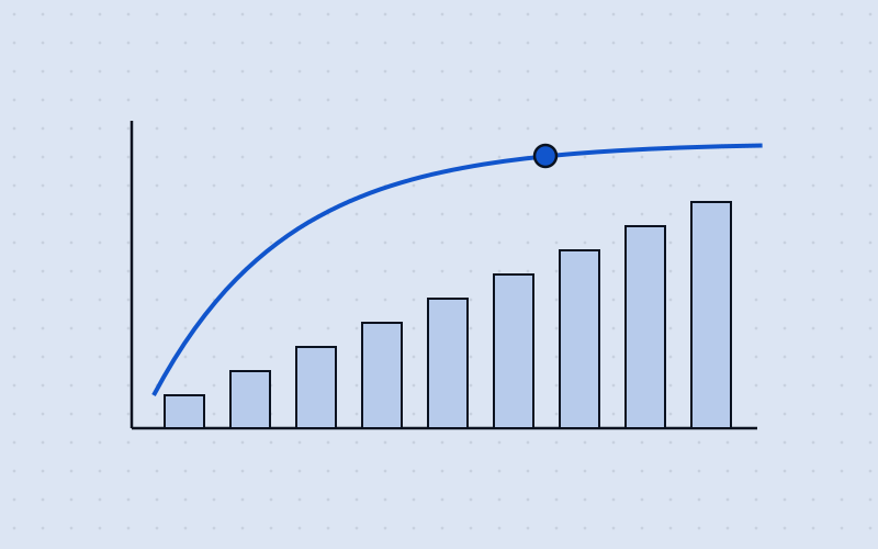
The pneumothorax learning curve is the direct answer to "do I need all the data at once?" Willemink and colleagues describe the same shape generally: performance on computer-vision tasks increases roughly logarithmically with training volume, which means each equal increment of accuracy costs multiplicatively more data than the last. The same paper notes that while generalizable algorithms may need datasets in the hundreds of thousands, relatively small datasets in the hundreds can be sufficient for specific targeted applications and populations. Narrowing the intended use is a legitimate way to reduce the data requirement, often the cheapest one available.
The Epic Sepsis Model is the answer to "is a lot of data enough?" A proprietary model deployed across hundreds of US hospitals, developed on very large volumes of operational EHR data, achieved an AUC of 0.63 and 33% sensitivity in external validation. Volume did not deliver transfer. Site-specific case mix, documentation practice, and label definition did.
Caveats
Proof-of-concept scale does not predict production-scale generalization. A research pediatric wrist-fracture model used 395 unique patients, split into 229 training, 41 tuning, and 125 test cases, and performed well. That demonstrates a narrow proof of concept can work with hundreds of cases. It says nothing about multi-site robustness or regulatory sufficiency. The right use of PoC evidence is as baseline evidence generation for later stages: it establishes label feasibility, an error taxonomy, a first learning curve, and a leakage check. It is not a scaled-down version of the pivotal study.
Training N is a property of the task, not of the calendar. Measure it with learning curves rather than declaring it in advance, and treat every published training-volume rule of thumb, including the opening estimates quoted in this article, as a negotiating figure to be replaced by your own curve.
The regulatory basis is sufficiency, independence, and claim coverage. Not volume. Three questions decide whether a dataset is adequate: is it sufficient in amount and quality for this device and intended purpose; is the test evidence genuinely independent of development at the patient, site, and acquisition levels the claim requires; and does the evidence cover every claim in the intended-use statement, including each subgroup, site type, device, and user population named in it. A dataset can be very large and fail all three.
Limits of the guidance in this article
- The stage table is a worked example, not a requirement, consensus standard, or legal advice. Its counts are arithmetic consequences of one assumed expected performance (0.90), one assumed prevalence (10%), a chosen half-width per stage for the estimation stages, and a chosen margin, alpha, and power for the hypothesis-test stages. Substitute your own and the whole table changes.
- The co-primary correction at stage 4 treats the sensitivity and specificity tests as independent, which is conservative: they are estimated on the same patients and are usually positively associated, so true joint power is somewhat higher than 90%.
- The binary precision calculations assume independent observations and use a normal approximation. Final sizing can differ under exact or Wilson intervals, hypothesis testing, Bayesian designs, clustering, repeated measures, multiple endpoints, adaptive designs, or negotiated acceptance criteria.
- Synthetic or augmented samples may improve training, but they are not additional independent clinical patients for pivotal evidence. Foundation-model pretraining can reduce task-specific label needs without removing the need for intended-use validation.
- The dermatology studies are illustrative. They include company-affiliated authors, mixed reference standards, an early evaluation whose study images partly entered training, and sparse darker-skin representation.
- Public FDA decision summaries are abbreviated and may omit training-set details.
- FDA, EU, UK, Canada, Japan, and other jurisdictions differ in classification, submission route, clinical-investigation requirements, and post-market obligations. Confirm the plan for each market.
- Evidence and guidance status were checked in August 2026. The FDA device-count figures reflect the March 2026 list update, NICE HTG746 was last updated in March 2026, and the FDA AI lifecycle guidance cited above remains draft.
Inputs needed to produce a defensible exact budget
A specific, defensible number requires all of the following, and it changes when any one of them changes.
Claim and context. The intended-use statement in one sentence: population, input, output, user, setting, and clinical action. Jurisdiction, device classification, and submission route. Whether the device is autonomous or assistive, and what happens when it is wrong. Whether the claim is analytical performance, diagnostic accuracy, reader improvement, management change, or patient outcome.
Statistics. Target-condition prevalence in the intended-use population, and whether the study will be natural-prevalence or enriched. Primary metric, expected performance or effect size, and the required confidence-interval width, non-inferiority margin, or power. Subgroups that must carry their own claim. Expected non-evaluable rate, attrition, clustering structure, and multiplicity.
Data and engineering. Modality, prediction unit, and the true unit of independence. Number of sites, acquisition systems, and operators in scope. Label and reference-standard process, including who adjudicates and how disagreement is resolved. Model class, and whether pretraining is available and licensable for commercial use. Failure-to-process policy. Legal basis for each dataset: consent, secondary use, commercial use, transfer, and retention for retraining.
Workflow. Clinical workflow, user groups, and the human-factors validation population. What the post-market monitoring window must be able to detect, and how quickly.
Recommended next steps
- Write the intended-use statement in one sentence: population, input, output, user, setting, and clinical action.
- Classify the risk of each false negative, false positive, failure-to-process result, and misuse scenario.
- Select one primary endpoint and a clinically justified acceptance threshold or comparison.
- Build a data-coverage matrix across site, time, device or scanner, demographics, disease spectrum, confounders, users, and failure modes.
- Reserve the locked test cohort by patient, site, and time before model and threshold selection.
- Fit learning curves and label-agreement curves; acquire more development data only where they show benefit or close a coverage gap.
- Calculate the pivotal sample from the endpoint, then inflate for prevalence, exclusions, clustering, multiplicity, and subgroup claims.
- Seek FDA Q-Submission, notified-body, PMDA, MHRA, or other jurisdiction-specific feedback before the pivotal protocol and design freeze.
- Maintain dataset lineage, consent and legal basis, annotation provenance, versioning, exclusions, and leakage checks under the quality system.
Step 9 is where most of the preceding eight quietly fail. A data budget only works if the organisation can prove what went into each dataset, when, from whom, under what permission, and with what label provenance, and can still prove it two years later when a modification needs sequestered test data. That is a tooling and process problem rather than a statistics problem, and it is the subject of the companion article on how MAEA solves the data lifecycle problem.
If your team is sizing a validation study or defending a data budget, ModAstera can review the endpoint, the sizing method, and the coverage matrix before recruitment starts.
References
Regulatory and study-design sources
- IMDRF N41: SaMD Clinical Evaluation
- IMDRF N88: Good Machine Learning Practice, final 2025
- MDCG 2020-1: Clinical Evaluation of Medical Device Software
- MDCG 2025-6 / AIB 2025-1: MDR, IVDR, and AI Act interplay
- FDA AI-enabled device lifecycle and submission recommendations, draft
- FDA final AI-enabled device PCCP guidance
- FDA statistical guidance for diagnostic-test studies
- FDA pivotal medical-device study design guidance
- FDA human factors and usability guidance
- FDA AI-Enabled Medical Device List
- PMDA SaMD review and consultation services
- NICE HTG746 recommendations for AI skin-lesion triage
Sample-size methods
- Buderer 1996: prevalence-aware sensitivity and specificity sample size
- Whittle et al. 2025: sample size for prediction models using a classification threshold
- Stark and Zapf 2020: prevalence-based sizing and re-estimation for confirmatory diagnostic accuracy
- Riley et al. 2021: minimum sample size for external validation with a binary outcome
- Snell et al. 2021: simulation-based sample size beats rules of thumb
- Wilson et al. 2022: Bayesian sample size determination for diagnostic accuracy studies
- Obuchowski and Bullen 2022: multireader diagnostic accuracy studies
- FDA iMRMC software for reader studies
- Monti, Ambrogi and Sardanelli 2024: sample size for data reliability and diagnostic performance
- Riley and Collins 2023: stability of clinical prediction models
- pmvalsampsize R package
Empirical and domain sources
- Kaushal, Altman and Langlotz 2020: geographic distribution of US training cohorts
- Willemink et al. 2020: preparing medical imaging data for machine learning
- IFCC machine-learning recommendations
- Pneumothorax classifier training-volume learning curves
- Pediatric wrist-fracture proof-of-concept study
- Wong et al. 2021: external validation of the Epic Sepsis Model
- Beede et al. 2020: human-centered evaluation of a deployed diabetic-retinopathy system
- Narang et al. 2021: deep-learning guidance for novice echocardiography
- DERM melanoma evaluation, JAMA Network Open 2019
- DERM-003 SCC/BCC study, Frontiers in Medicine 2023
- DERM teledermatology impact study, Frontiers in Medicine 2024
- Diverse Dermatology Images external evaluation
- MedTech Dive AI device tracker, March 2026 FDA list update